Choosing the Right PostgreSQL Index, a Practical Guide
Table of Contents
Comparison of commonly used index types in PostgreSQL and when to (and when not to) choose them.
No one would argue against the benefits of indexing, but misuse can cause a lot of headaches, particularly in high-traffic environments. Two of the most common index-related mistakes I see are over-indexing and choosing the wrong index type. The former becomes particularly painful when an enthusiastic engineer indexes every single column on a write-heavy table. The next thing you see is index bloat, with your database server struggling to keep autovacuum running. Over-indexing is too workload-specific for a general guide like this, but choosing the wrong index type is something we can talk about.
The idea of this article is not to show you which index types are out there, but to share the common applications and index types you could use to have indexes work for you rather than against you. We will go through the three index types that cover most use cases, starting with the easiest to understand.
Why You Probably Won’t Need Hash Indexes #
Hash indexes are PostgreSQL’s one-trick pony. They support only equality and that’s it. No ranges, ordering, uniqueness constraints or multi-column composites. No NULL searches since NULL values aren’t supported by equality operators. For most application use cases, these are enough to never use them.
-- Demo table
CREATE TABLE tickets (
    ticket_no       char(13)    PRIMARY KEY,
    book_ref        char(6)     NOT NULL,
    passenger_id    varchar(20) NOT NULL,
    passenger_name  text,
    contact_data    jsonb
);

CREATE INDEX tickets_passenger_id_hash
    ON tickets USING hash (passenger_id);
Hashing mechanics are straightforward: Postgres hashes the column value with an internal hash_any function into a 4-byte integer, regardless of input size. Equality-only support combined with the narrow case of large-value columns is what keeps Hash indexes useful.
One small advantage is the “slightly” narrower footprint compared to B-trees. The gap here is less than the 4-byte integer would make you think. B-trees use tricks like deduplication and suffix truncation to compress storage, while Hash entries themselves carry overhead, with each one including a 6-byte TID alongside the 4-byte hash.
So, even if you have high cardinality columns with large values, B-trees could still be the safer bet since the slightly larger footprint is more than paid for by the features you get in return.
B-tree: The Default #
If you’re not sure which index to use, B-tree is most likely what you need. It’s the access method behind primary keys, unique constraints, and the vast majority of indexes.
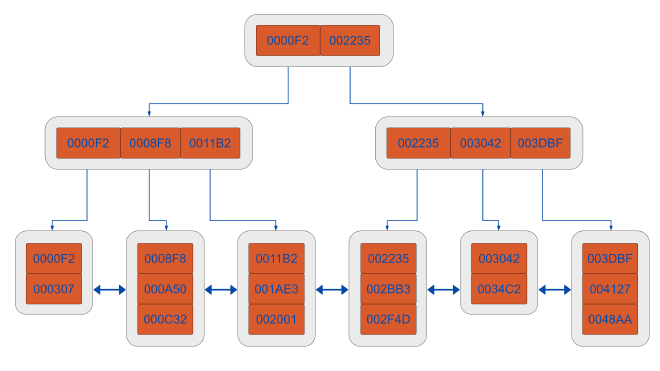
The structure is a balanced search tree. Lookups traverse from a root page through internal pages down to leaf pages that store the indexed values and row pointer TIDs. Internal pages hold sorted separator keys that route the search.
The descent is O(log n) and because leaf pages are doubly linked, range scans walk sideways through them without re-traversing the tree. This is how B-tree supports =, <, <=, >, >=, BETWEEN, prefix LIKE 'foo%', and ORDER BY with one index structure.
The operators are linked via a B-tree operator family, and the five strategies (<, <=, =, >=, >) are mandatory. In other words a type without all five can’t have a B-tree opclass. You can list them for any type:
SELECT amopopr::regoperator AS operator,
       amopstrategy
  FROM pg_am am
  JOIN pg_opfamily opf ON opf.opfmethod = am.oid
  JOIN pg_amop amop    ON amop.amopfamily = opf.oid
 WHERE am.amname  = 'btree'
   AND opf.opfname = 'integer_ops'
 ORDER BY amopstrategy;


       operator        | amopstrategy
-----------------------+--------------
 <(integer,integer)    |            1
 <=(integer,integer)   |            2
 =(integer,integer)    |            3
 >=(integer,integer)   |            4
 >(integer,integer)    |            5
A typical setup using a flight booking schema:
CREATE INDEX tickets_book_ref_idx ON tickets (book_ref);
CREATE INDEX tickets_name_idx ON tickets (passenger_name);
ANALYZE tickets;
NULL values are stored and sortable in B-tree, and by default they sort greater than any non-null, which you can flip per-index with NULLS FIRST (or per-query with ORDER BY).
Deduplication collapses repeated key values into a single entry pointing to a posting list of TIDs. It’s enabled by default and significantly reduces index size on low-cardinality columns. To check whether a specific index has it on:
SELECT relname, reloptions
  FROM pg_class
 WHERE relname = 'tickets_book_ref_idx';
A deduplicate_items=off in reloptions means it’s been disabled. Absent or on means it’s enabled, which is the default.
Another interesting property: B-trees are clusterable. CLUSTER tickets USING tickets_book_ref_idx physically reorders the heap to match the index. The correlation isn’t maintained on future writes, but it’s useful for read-heavy tables.
Now let’s take a quick look at commonly used index scans in B-tree indexes.
Common Scan Types in B-tree Indexes #
The planner picks an execution strategy based on selectivity, the columns the query needs, and how scattered the matching rows are likely to be on disk.
Index Scan is straightforward. It descends the tree, finds matching keys, and follows each TID back to the heap to fetch the row, with one heap visit per match. This is the default for highly selective queries like primary key or unique column lookups.
tickets=# EXPLAIN (ANALYZE, BUFFERS) SELECT * FROM tickets WHERE book_ref = '00DC4F';
                                                            QUERY PLAN
-----------------------------------------------------------------------------------------------------------------------------------
 Index Scan using tickets_book_ref_idx on tickets  (cost=0.29..8.31 rows=1 width=114) (actual time=0.038..0.038 rows=0.00 loops=1)
   Index Cond: (book_ref = '00DC4F'::bpchar)
   Index Searches: 1
   Buffers: shared read=2
 Planning:
   Buffers: shared hit=17 read=2
 Planning Time: 0.307 ms
 Execution Time: 0.071 ms
(8 rows)
Bitmap Heap Scan (runs on top of a Bitmap Index Scan) walks the index first and builds an in-memory bitmap of the matching heap pages. A second pass visits these pages in physical order, converting random I/O into sequential I/O. The planner chooses this type on medium selectivity queries (approximately 1% to 20% of the table). It is also used when combining two indexes via BitmapAnd or BitmapOr.
tickets=# EXPLAIN (ANALYZE, BUFFERS) SELECT * FROM tickets WHERE passenger_name = 'JOHN SMITH';
                                                            QUERY PLAN
----------------------------------------------------------------------------------------------------------------------------------
 Bitmap Heap Scan on tickets  (cost=11.71..969.45 rows=957 width=114) (actual time=0.605..5.383 rows=1000.00 loops=1)
   Recheck Cond: (passenger_name = 'JOHN SMITH'::text)
   Heap Blocks: exact=909
   Buffers: shared hit=909 read=2
   ->  Bitmap Index Scan on tickets_name_idx  (cost=0.00..11.47 rows=957 width=0) (actual time=0.449..0.450 rows=1000.00 loops=1)
         Index Cond: (passenger_name = 'JOHN SMITH'::text)
         Index Searches: 1
         Buffers: shared read=2
 Planning Time: 0.310 ms
 Execution Time: 5.626 ms
(10 rows)
Index Only Scan skips the heap entirely when every column the query needs is in the index. It still has to confirm row visibility, which it does via the visibility map rather than the heap, so the optimisation depends on the table being well vacuumed. Because it avoids the heap visit altogether, it does the least I/O of the three scan types, which makes it the fastest path and the one to aim for on low-latency queries.
You can verify it’s working by the Heap Fetches: line in the plan above. A non-zero value means it’s falling back to the heap and losing the benefit.
tickets=# EXPLAIN (ANALYZE, BUFFERS) SELECT book_ref FROM tickets WHERE book_ref BETWEEN '00A000' AND '00B000';
                                                              QUERY PLAN
---------------------------------------------------------------------------------------------------------------------------------------
 Index Only Scan using tickets_book_ref_idx on tickets  (cost=0.29..4.33 rows=2 width=7) (actual time=0.023..0.025 rows=11.00 loops=1)
   Index Cond: ((book_ref >= '00A000'::bpchar) AND (book_ref <= '00B000'::bpchar))
   Heap Fetches: 0
   Index Searches: 1
   Buffers: shared hit=3
 Planning:
   Buffers: shared hit=6
 Planning Time: 0.214 ms
 Execution Time: 0.047 ms
(9 rows)
GIN: Stop B-tree Indexing your jsonb #
Where B-tree treats each indexed value as a single comparable unit, GIN (Generalised Inverted Index) looks inside a field and indexes its components. This is particularly useful where one row contains many searchable items: array elements, tsvector lexemes or the key-value pairs inside a jsonb document.
jsonb is widely used in web applications for things like storing user preferences, device metadata, webhook payloads or contact details. The problem occurs when the application queries the document contents. A B-tree is pointless here, since it would only match on whole-document equality. GIN is what makes a clause like WHERE contact_data @> '...' to actually use an index.
Let’s build an example index and query on the contact_data field:
CREATE INDEX tickets_contact_data_gin
    ON tickets USING gin (contact_data);

SELECT ticket_no, passenger_name
  FROM tickets
 WHERE contact_data @> '{"email": "[email protected]"}';
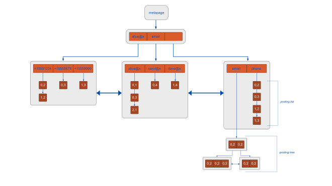
GIN (as the name suggests) gets built as an inverted index. For jsonb, it uses the jsonb_ops opclass. Each key and each value in the document gets extracted as its own index entry. Each extracted item maps to a posting list of TIDs for the rows that contain it. Given a key or value to search for, GIN jumps straight to the matching rows without scanning the heap.
The jsonb_ops class supports the common search operators:
SELECT * FROM tickets WHERE contact_data @> '{"phone":"+15551234"}';
SELECT * FROM tickets WHERE contact_data ? 'email';
SELECT * FROM tickets WHERE contact_data ?| array['phone','fax'];
SELECT * FROM tickets WHERE contact_data ?& array['phone','email'];
The four operators listed above are:
- containment:
@> - top-level key existence:
? - any of these keys:
?| - all of these keys:
?&
One small hint is using jsonb_path_ops for applications that only use containment (@>). This opclass uses a smaller index by hashing whole key-value paths instead of indexing each key and value separately.
CREATE INDEX tickets_contact_data_path_gin
    ON tickets USING gin (contact_data jsonb_path_ops);
For this index type, the other three operators will fall back to a sequential scan if this is the only index available.